• Skip to main content
  • Skip to primary sidebar

学習記録

機械学習

機械学習用データの用意(ランダムデータで散布図)

2017年12月13日 by 河副 太智 Leave a Comment

1
2
3
4
5
6
7
8
9
10
11
12
13
14
15
16
17
18
19
20
21
22
23
24
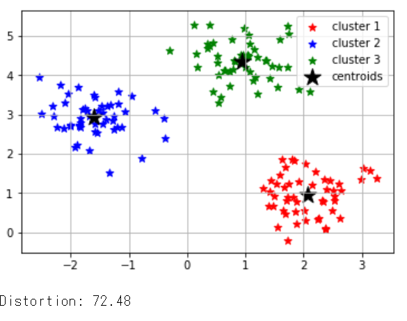
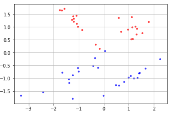
様々な分類の手法について実際にコードを動かして学ぶ際に、分類ができそうなデータを用意する必要があります。
実用レベルでは実際に測定された何かしらの値を入手するところから始めますが、今回はその部分は省き、架空の分類用データを自分で作成してしまいましょう。
分類に適したデータを作成するには、scikit-learn.datasetsモジュールのmake_classification() 関数を使います。
 
make_classificationの引数
 
# モジュールのimport
from sklearn.datasets import make_classification
# データX, ラベルyの生成
X, y = make_classification(n_samples, n_classes, n_features, n_redundant, random_state)
上記関数の各引数は以下のとおりです
n_samples
用意するデータの個数
n_classes
クラス数。デフォルトは2
n_features
データの特徴量の個数
n_redundant
分類に不要な特徴量(余分な特徴量)の個数
random_state
乱数のシード(乱数のパターンを決定する要素)
他にも引数はありますが、この章ではこれらを定義したデータを作成していきます。  
また、データがどのクラスに属しているかを示す「ラベル(y)」が用意されますが、基本的に整数値によってラベルを用意します。  
例えば二項分類であれば各データのラベルは「0」または「1」になります。

  • n_classes
    クラス数。デフォルトは2
  • n_features
    データの特徴量の個数
  • n_redundant
    分類に不要な特徴量(余分な特徴量)の個数
  • random_state
    乱数のシード(乱数のパターンを決定する要素)


1
2
3
4
5
6
7
8
9
10
11
12
13
14
15
16
# モジュールのimport
from sklearn.datasets import make_classification
# プロット用モジュール
import matplotlib.pyplot as plt
import matplotlib
%matplotlib inline
 
 
# コード
# データX, ラベルyを生成
X, y = make_classification(n_samples=50, n_features=2, n_redundant=0, random_state=0)
 
# データの色付け、プロット
plt.scatter(X[:, 0], X[:, 1], c=y, marker='.',
cmap=matplotlib.cm.get_cmap(name='bwr'), alpha=0.7)
plt.grid(True)


1
2
3
他にも引数はありますが、この章ではこれらを定義したデータを作成していきます。  
また、データがどのクラスに属しているかを示す「ラベル(y)」が用意されますが、基本的に整数値によってラベルを用意します。  
例えば二項分類であれば各データのラベルは「0」または「1」になります。

Filed Under: グラフ, 機械学習

SSEとエルボー法

2017年12月12日 by 河副 太智 Leave a Comment


クラスタリングの性能評価関数にSSE(クラスタ内誤差平方和)がある
SSEにより様々なk-meansクラスタリングの性能を評価可能。

SSEの式
print(‘Distortion: %.2f’% km.inertia_)

クラスタ内誤差平方和を出力、クラスターの数を調整して一番低いものが正確


1
 

1
2
3
4
5
6
7
8
9
10
11
12
13
14
15
16
17
18
19
20
21
22
23
24
25
26
27
28
29
30
31
32
33
34
35
36
37
38
39
40
41
42
43
44
45
46
47
48
49
50
51
52
53
import matplotlib.pyplot as plt
import numpy as np
import pandas as pd
 
from sklearn.cluster import KMeans
from sklearn.datasets import make_blobs
 
# Xには1つのプロットの(x,y)が、yにはそのプロットの所属するクラスター番号が入る
X,y = make_blobs(n_samples=150,         # サンプル点の総数
               n_features=2,          # 特徴量(次元数)の指定  default:2
               centers=3,             # クラスタの個数
               cluster_std=0.5,       # クラスタ内の標準偏差
               shuffle=True,          # サンプルをシャッフル
               random_state=0)        # 乱数生成器の状態を指定
 
km = KMeans(n_clusters=3,        # クラスターの個数
            init='k-means++',           # セントロイドの初期値をランダムに設定  default: 'k-means++'
            n_init=10,               # 異なるセントロイドの初期値を用いたk-meansの実行回数
            max_iter=300,            # k-meansアルゴリズムを繰り返す最大回数
            tol=1e-04,               # 収束と判定するための相対的な許容誤差
            random_state=0)          # 乱数発生初期化
 
y_km = km.fit_predict(X) # クラスターが存在するデータを渡し、各サンプルに対するクラスタ番号を求める
 
plt.scatter(X[y_km==0,0],         # y_km(クラスター番号)が0の時にXの0列目を抽出
                    X[y_km==0,1], # y_km(クラスター番号)が0の時にXの1列目を抽出
                    s=50,
                    c='r',
                    marker='*',
                    label='cluster 1')
plt.scatter(X[y_km==1,0],
                    X[y_km==1,1],
                    s=50,
                    c='b',
                    marker='*',
                    label='cluster 2')
plt.scatter(X[y_km==2,0],
                   X[y_km==2,1],
                    s=50,
                    c='g',
                    marker='*',
                    label='cluster 3')
plt.scatter(km.cluster_centers_[:,0],   # km.cluster_centers_には各クラスターのセントロイドの座標が入っている
                    km.cluster_centers_[:,1],
                    s=250,
                    marker='*',
                    c='black',
                    label='centroids')
plt.legend(loc="best")
plt.grid()
plt.show()
 
print('Distortion: %.2f'% km.inertia_) #クラスタ内誤差平方和を出力、クラスターの数を調整して一番低いものが正確


しかし、この方法だと一度に一つのクラスタだけしか評価できないのでエルボー法により
forを10回回して10個分のSSEをグラフに表示させ、急降下している部分を見つける事が可能


1
2
3
4
5
6
7
8
9
10
11
12
13
14
15
16
17
18
19
20
21
22
23
24
25
26
27
28
29
30
31
32
33
34
35
36
37
38
39
import matplotlib.pyplot as plt
import numpy as np
import pandas as pd
 
from sklearn.cluster import KMeans
from sklearn.datasets import make_blobs
 
# Xには1つのプロットの(x,y)が、yにはそのプロットの所属するクラスター番号が入る
X,y = make_blobs(n_samples=150,         # サンプル点の総数
               n_features=2,          # 特徴量(次元数)の指定  default:2
               centers=3,             # クラスタの個数
               cluster_std=0.5,       # クラスタ内の標準偏差
               shuffle=True,          # サンプルをシャッフル
               random_state=0)        # 乱数生成器の状態を指定
 
km = KMeans(n_clusters=3,        # クラスターの個数
            init='k-means++',           # セントロイドの初期値をランダムに設定  default: 'k-means++'
            n_init=10,               # 異なるセントロイドの初期値を用いたk-meansの実行回数
            max_iter=300,            # k-meansアルゴリズムを繰り返す最大回数
            tol=1e-04,               # 収束と判定するための相対的な許容誤差
            random_state=0)          # 乱数発生初期化
 
y_km = km.fit_predict(X) # クラスターが存在するデータを渡し、各サンプルに対するクラスタ番号を求める
 
distortions = []
 
for i  in range(1,11):                # 1~10クラスタまで一気に計算
    km = KMeans(n_clusters=i,
                init='k-means++',     # k-means++法によりクラスタ中心を選択
                n_init=10,
                max_iter=300,
                random_state=0)
    km.fit(X)                         # クラスタリングの計算を実行
    distortions.append(km.inertia_)   # km.fitするとkm.inertia_が得られる
 
plt.plot(range(1,11),distortions,marker='o')
plt.xlabel('Number of clusters')
plt.ylabel('Distortion')
plt.show()


Filed Under: 機械学習

k-means

2017年12月12日 by 河副 太智 Leave a Comment

k-means法でのクラスタリング


1
2
3
4
5
6
7
8
9
10
11
12
13
14
15
16
17
18
19
20
21
22
23
24
25
26
27
28
29
30
31
32
33
34
35
36
37
38
39
40
41
import matplotlib.pyplot as plt
import numpy as np
 
from sklearn.cluster import KMeans
from sklearn.datasets import make_blobs
 
# Xには1つのプロットの(x,y)が、yにはそのプロットの所属するクラスター番号が入る
X,y = make_blobs(n_samples=150,         # サンプル点の総数
               n_features=2,          # 特徴量(次元数)の指定  default:2
               centers=3,             # クラスタの個数
               cluster_std=0.5,       # クラスタ内の標準偏差
               shuffle=True,          # サンプルをシャッフル
               random_state=0)        # 乱数生成器の状態を指定
 
km = KMeans(n_clusters=3, random_state=0)
y_km = km.fit_predict(X)
 
fig, (ax1, ax2) = plt.subplots(1, 2, figsize=(8,3))
 
ax1.scatter(X[:, 0],
            X[:, 1],
            c='black')
ax1.grid()
 
ax2.scatter(X[y_km==0, 0],
            X[y_km==0, 1],
            c='r',
            s=40,
            label='cluster 1')
ax2.scatter(X[y_km==1, 0],
            X[y_km==1, 1],
            c='b',
            s=40,
            label='cluster 2')
ax2.scatter(X[y_km==2, 0],
            X[y_km==2, 1],
            c='g',
            s=40,
            label='cluster 3')
ax2.grid()
plt.show()


Filed Under: 機械学習

クラスタリングとデンドログラフ

2017年12月12日 by 河副 太智 Leave a Comment

階層的クラスタリング、デンドログラフという階層を持つ

非階層的クラスタリングも、階層的クラスタリングと同じように
データから似た性質の法則を探し出し、クラスターを作るが階層構造を持たない。


非階層的クラスタリングはクラスターの数を開発者が決める
大量のデータを扱うのにてきしており、k-means法が使われる


1
2
3
4
5
6
7
8
9
10
11
12
13
14
15
16
17
import matplotlib.pyplot as plt
import numpy as np
import pandas as pd
 
from sklearn.datasets import make_blobs
 
# Xには1つのプロットの(x,y)が、yにはそのプロットの所属するクラスター番号が入る
X,y = make_blobs(n_samples=500,         # サンプル点の合計
               n_features=2,          # 特徴量の指定  次元数とも呼ぶ
               centers=3,             # クラスタの個数
               cluster_std=0.5,       # クラスタ内の標準偏差
               shuffle=True,          # シャッフル
               random_state=0)        # 乱数生成器を指定
 
plt.scatter(X[:,0], X[:,1], c='red', marker='*', s=50) #下のサンプルはblack
plt.grid()
plt.show()


Filed Under: 機械学習

線形重回帰

2017年12月7日 by 河副 太智 Leave a Comment

1
2
3
4
5
6
7
8
9
10
11
12
13
14
15
from sklearn.linear_model import LinearRegression
from sklearn.datasets import make_regression
from sklearn.model_selection import train_test_split
 
# データ生成
X, y = make_regression(n_samples=100, n_features=10, n_informative=3, n_targets=1, noise=5.0, random_state=42)
train_X, test_X, train_y, test_y = train_test_split(X, y, random_state=42)
 
 
# モデル構築
model = LinearRegression()
# 学習
model.fit(train_X, train_y)
# test_Xへの推測結果
print(model.predict(test_X))


Filed Under: 機械学習

回帰3種類[線形、ラッソ、リッジ]

2017年12月7日 by 河副 太智 Leave a Comment

線形単回帰とは予測したいデータと予測に使用するデータが一つづつとなる回帰分析
データ同士の関連性を示す

予測したいデータをyとすると予測用データをxとすると
y = ax + b


の関係性を仮定しaとbを最小二乗法という方法で分析

yの値と推定するy=ax+bの差の二乗の総和が最小となるaとbを算出

この手法はscikit-learnのlinear_modelモジュールの
LinearRegressionを使用して回帰分析を行う


■線形回帰

1
2
3
4
5
6
7
8
9
10
11
12
13
14
15
16
from sklearn.linear_model import LinearRegression
from sklearn.datasets import make_regression
from sklearn.model_selection import train_test_split
 
# データ生成
X, y = make_regression(n_samples=100, n_features=1, n_targets=1, noise=5.0, random_state=42)
train_X, test_X, train_y, test_y = train_test_split(X, y, random_state=42)


# 線形回帰モデル構築
model = LinearRegression()
# 学習
model.fit(train_X, train_y)
# 係数の出力
print(model.score(test_X, test_y))


■リッジ回帰

1
2
3
4
5
# リッジ回帰モデル
model = Ridge()
model.fit(train_X, train_y)
# test_X, test_yに対する決定係数を出力してください
print("リッジ回帰:{}".format(model.score(test_X, test_y)))


■ラッソ回帰

1
2
3
4
5
# ラッソ回帰モデル(データ生成は線形回帰を参照)
model = Lasso()
model.fit(train_X, train_y)
# test_X, test_yに対する決定係数を出力してください
print("ラッソ回帰:{}".format(model.score(test_X, test_y)))


Filed Under: 機械学習 Tagged With: ラッソ回帰, リッジ回帰, 線形回帰

  • « Go to Previous Page
  • Page 1
  • Interim pages omitted …
  • Page 6
  • Page 7
  • Page 8
  • Page 9
  • Go to Next Page »

Primary Sidebar

カテゴリー

  • AWS
  • Bootstrap
  • Dash
  • Django
  • flask
  • GIT(sourcetree)
  • Plotly/Dash
  • VPS
  • その他tool
  • ブログ
  • プログラミング
    • Bokeh
    • css
    • HoloViews
    • Jupyter
    • Numpy
    • Pandas
    • PosgreSQL
    • Python 基本
    • python3
      • webアプリ
    • python3解説
    • scikit-learn
    • scipy
    • vps
    • Wordpress
    • グラフ
    • コマンド
    • スクレイピング
    • チートシート
    • データクレンジング
    • ブロックチェーン
    • 作成実績
    • 時系列分析
    • 機械学習
      • 分析手法
      • 教師有り
    • 異常値検知
    • 自然言語処理
  • 一太郎
  • 数学
    • sympy
      • 対数関数(log)
      • 累乗根(n乗根)
    • 暗号学

Copyright © 2025 · Genesis Sample on Genesis Framework · WordPress · Log in