• Skip to main content
  • Skip to primary sidebar

学習記録

プログラミング

クラスタリングとデンドログラフ

2017年12月12日 by 河副 太智 Leave a Comment

階層的クラスタリング、デンドログラフという階層を持つ

非階層的クラスタリングも、階層的クラスタリングと同じように
データから似た性質の法則を探し出し、クラスターを作るが階層構造を持たない。


非階層的クラスタリングはクラスターの数を開発者が決める
大量のデータを扱うのにてきしており、k-means法が使われる


1
2
3
4
5
6
7
8
9
10
11
12
13
14
15
16
17
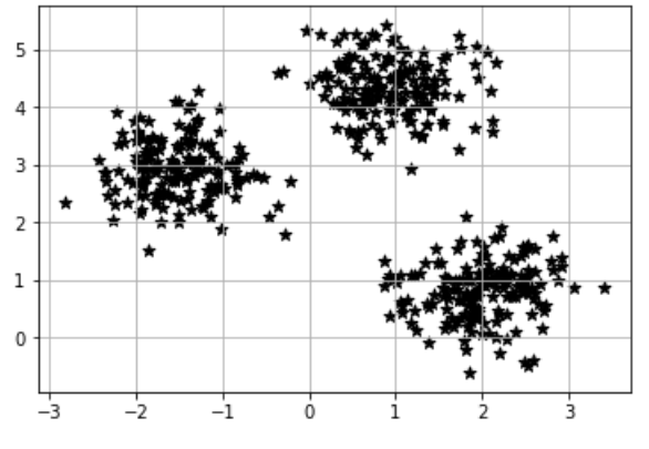
import matplotlib.pyplot as plt
import numpy as np
import pandas as pd
 
from sklearn.datasets import make_blobs
 
# Xには1つのプロットの(x,y)が、yにはそのプロットの所属するクラスター番号が入る
X,y = make_blobs(n_samples=500,         # サンプル点の合計
               n_features=2,          # 特徴量の指定  次元数とも呼ぶ
               centers=3,             # クラスタの個数
               cluster_std=0.5,       # クラスタ内の標準偏差
               shuffle=True,          # シャッフル
               random_state=0)        # 乱数生成器を指定
 
plt.scatter(X[:,0], X[:,1], c='red', marker='*', s=50) #下のサンプルはblack
plt.grid()
plt.show()


Filed Under: 機械学習

線形重回帰

2017年12月7日 by 河副 太智 Leave a Comment

1
2
3
4
5
6
7
8
9
10
11
12
13
14
15
from sklearn.linear_model import LinearRegression
from sklearn.datasets import make_regression
from sklearn.model_selection import train_test_split
 
# データ生成
X, y = make_regression(n_samples=100, n_features=10, n_informative=3, n_targets=1, noise=5.0, random_state=42)
train_X, test_X, train_y, test_y = train_test_split(X, y, random_state=42)
 
 
# モデル構築
model = LinearRegression()
# 学習
model.fit(train_X, train_y)
# test_Xへの推測結果
print(model.predict(test_X))


Filed Under: 機械学習

回帰3種類[線形、ラッソ、リッジ]

2017年12月7日 by 河副 太智 Leave a Comment

線形単回帰とは予測したいデータと予測に使用するデータが一つづつとなる回帰分析
データ同士の関連性を示す

予測したいデータをyとすると予測用データをxとすると
y = ax + b


の関係性を仮定しaとbを最小二乗法という方法で分析

yの値と推定するy=ax+bの差の二乗の総和が最小となるaとbを算出

この手法はscikit-learnのlinear_modelモジュールの
LinearRegressionを使用して回帰分析を行う


■線形回帰

1
2
3
4
5
6
7
8
9
10
11
12
13
14
15
16
from sklearn.linear_model import LinearRegression
from sklearn.datasets import make_regression
from sklearn.model_selection import train_test_split
 
# データ生成
X, y = make_regression(n_samples=100, n_features=1, n_targets=1, noise=5.0, random_state=42)
train_X, test_X, train_y, test_y = train_test_split(X, y, random_state=42)


# 線形回帰モデル構築
model = LinearRegression()
# 学習
model.fit(train_X, train_y)
# 係数の出力
print(model.score(test_X, test_y))


■リッジ回帰

1
2
3
4
5
# リッジ回帰モデル
model = Ridge()
model.fit(train_X, train_y)
# test_X, test_yに対する決定係数を出力してください
print("リッジ回帰:{}".format(model.score(test_X, test_y)))


■ラッソ回帰

1
2
3
4
5
# ラッソ回帰モデル(データ生成は線形回帰を参照)
model = Lasso()
model.fit(train_X, train_y)
# test_X, test_yに対する決定係数を出力してください
print("ラッソ回帰:{}".format(model.score(test_X, test_y)))


Filed Under: 機械学習 Tagged With: ラッソ回帰, リッジ回帰, 線形回帰

機械学習 ワイン

2017年12月7日 by 河副 太智 Leave a Comment

1
2
3
4
5
6
7
8
9
10
11
12
13
14
15
16
17
18
19
# 必要モジュールをインポート
from sklearn.linear_model import LinearRegression
from sklearn.datasets import load_wine
from sklearn.model_selection import train_test_split
 
 
data = load_wine()
# データを教師用とテスト用に
train_X, test_X, train_y, test_y = train_test_split(
    data.data, data.target, random_state=42)
print(data)
# 学習器の構築
model = LinearRegression()
# 教師データを用いて学習器に学習
model.fit(train_X, train_y)
# テスト用データを用いて学習結果をpred_yに代入
pred_y = model.predict(test_X)
# 予測結果を出力
#print(pred_y)


Filed Under: 機械学習

円グラフ

2017年12月7日 by 河副 太智 Leave a Comment


1
2
3
4
5
6
7
8
9
10
11
12
import matplotlib.pyplot as plt
%matplotlib inline
 
 
data = [60, 20, 10, 5, 3, 2]
labels = ['Apple', 'Orange', 'Banana', 'Pineapple', 'Kiwifruit', 'Strawberry']
explode = [0, 0, 0.1, 0, 0, 0]
 
# dataにlabelsのラベルをつけて、Bananaを目立たせた円グラフ可視化
plt.pie(data, labels=labels, explode=explode)
plt.axis('equal')
plt.show()

explodeは目立たせたい円グラフを0から1までの値でグラフから飛びだたせる

Filed Under: グラフ

散布図

2017年12月6日 by 河副 太智 Leave a Comment

1
2
3
4
5
6
7
8
9
10
11
12
import numpy as np
import matplotlib.pyplot as plt
%matplotlib inline
 
 
np.random.seed(0)
x = np.random.choice(np.arange(100), 100)
y = np.random.choice(np.arange(100), 100)
 
# マーカー色を設定して散布図を作成
plt.scatter(x, y, marker="s", color="r")
plt.show()


マーカー (,marker=”o”)

  • "o": 円
  • "s": 四角
  • "p": 五角形
  • "*": 星
  • "+": プラス
  • "D": ダイアモンド

色 (markerfacecolor=”r”)

  • "b" : 青
  • "g" : 緑
  • "r" : 赤
  • "c" : シアン
  • "m" : マゼンタ
  • "y" : 黄色
  • "k" : 黒
  • "w" : 白

Filed Under: グラフ

  • « Go to Previous Page
  • Page 1
  • Interim pages omitted …
  • Page 29
  • Page 30
  • Page 31
  • Page 32
  • Page 33
  • Interim pages omitted …
  • Page 55
  • Go to Next Page »

Primary Sidebar

カテゴリー

  • AWS
  • Bootstrap
  • Dash
  • Django
  • flask
  • GIT(sourcetree)
  • Plotly/Dash
  • VPS
  • その他tool
  • ブログ
  • プログラミング
    • Bokeh
    • css
    • HoloViews
    • Jupyter
    • Numpy
    • Pandas
    • PosgreSQL
    • Python 基本
    • python3
      • webアプリ
    • python3解説
    • scikit-learn
    • scipy
    • vps
    • Wordpress
    • グラフ
    • コマンド
    • スクレイピング
    • チートシート
    • データクレンジング
    • ブロックチェーン
    • 作成実績
    • 時系列分析
    • 機械学習
      • 分析手法
      • 教師有り
    • 異常値検知
    • 自然言語処理
  • 一太郎
  • 数学
    • sympy
      • 対数関数(log)
      • 累乗根(n乗根)
    • 暗号学

Copyright © 2025 · Genesis Sample on Genesis Framework · WordPress · Log in